
5. Architecture Implementation#
5.1. Required files#
5.2. Introduction#
This tutorial presents SpaceStudio’s Architecture Implementation functionality with a simple application. The application will be thoroughly explained in the next section.
Architecture implementation is the part of the SpaceStudio environment that implements or synthesizes your system for your preferred Computer Aided-Design (CAD) or Electronic Design Automation (EDA) implementation tool.
This tutorial is divided into two sections. In the first section, the attendee will use the provided architecture. The attendee will simulate the given architecture at the system architecture level, and then implement it on an FPGA using the architecture implementation feature.
In the concluding section of this tutorial, the attendee will create a new system architecture with a dedicated soft-core coprocessor for the computation modules. The new architecture will be simulated in the simulation environment and implemented on an FPGA using the architecture implementation feature.
Important
The EDA and the HLS tools used by the Architecture Implementation need to be installed and, if applicable, a valid license for them is required. In this tutorial, the HLS tool used is Vitis HLS, and the EDA tool used is Vivado, both developed by Xilinx. These tools require a license.
5.3. Application#
The application is a 32-bit unsigned integer calculator. Figure 5.5 presents the application’s flow. In the figure, there are 7 modules, each with one input and one output. In general, the data/command is sent by a host computer via a terminal. The data/command enters the application at the left of the figure. The Input Reader module reads the data/command and forwards it to the Controller. The Controller is responsible for decoding each operand and operation. The Controller enables the proper operation module by sending both operands and then waits for the result. The Controller takes the result and sends it to the Output Writer, and the result data exits the application flow at the right of the figure. In general, the result is read from a computer host via a terminal.
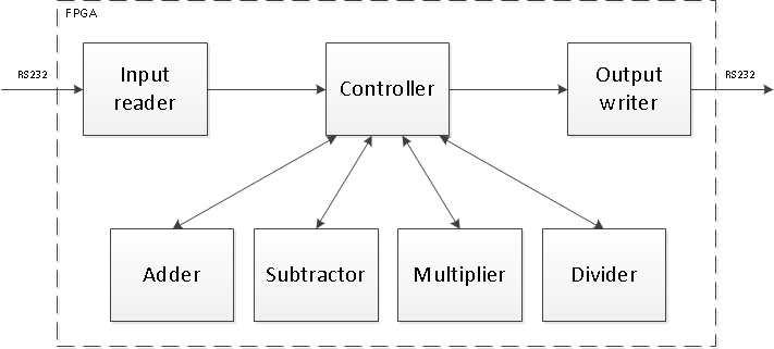
Figure 5.5 Calculator Application data flow#
5.3.1. Modules#
5.3.1.1. Input Reader#
5.3.1.1.1. Description#
The input_reader module is responsible for abstracting the communication layer from the computation layer. This enables designers to change I/O peripherals without changing the application. In other words, for this case, it transforms the RS232 communication into a FIFO-based communication.
5.3.1.1.2. Behaviour#
This module polls the UART for data. When data becomes available, it reads the data from the UART and sends the data to the controller through a FIFO.
5.3.1.2. Output Writer#
5.3.1.2.1. Description#
The output_writer module is responsible for abstracting the communication layer from the computation layer. This enables designers to change I/O peripherals without changing the application. In other words, for this case, it transforms a FIFO-based communication into an RS232 communication.
5.3.1.2.2. Behaviour#
This module waits for data sent by the controller. When no data is present in the FIFO, this module goes into a dormant state until data becomes available in the FIFO. When data is inserted into the FIFO by the controller, this module wakes up from an interrupt launched by the FIFO. It then reads the data from the FIFO and sends it to the UART.
5.3.1.3. Controller#
5.3.1.3.1. Description#
The controller is responsible for decoding each operand and the operation from the string obtained by the input_reader. The controller will only process valid strings. It forwards the execution of the operation to the proper module and waits for the result. The result is sent to the output_writer.
5.3.1.3.2. Behaviour#
This module waits for data sent by the input_reader. When no data is present in the FIFO, this module goes into a dormant state until data becomes available in the FIFO. When data is inserted into the FIFO by the input_reader, this module wakes up from an interrupt launched by the FIFO. It then reads the data from the FIFO. The input data is stored into an array of fixed length. If the input data overflows the array, a message is thrown. The controller stops storing data into the array when a line feed or carriage return character is detected. This array is then evaluated for correctness. If the input string is invalid, a message is thrown. If the input string is valid, the controller decodes each operand and the operation. The controller sends both operands to the proper module (adder, subtractor, multiplier or divider) and waits for the result. When the result becomes available, the controller forwards the result to the output_writer.
5.3.1.4. Adder#
5.3.1.4.1. Description#
The adder is responsible for performing the addition of two numbers and returns the result to the controller. The addition operation is denoted by the character '+'.
5.3.1.4.2. Behaviour#
This module waits for data sent by the controller. When no data is present in the FIFO, this module goes into a dormant state until data becomes available in the FIFO. When data is inserted into the FIFO by the controller, this module wakes up from an interrupt launched by the FIFO. It then reads the data from the FIFO. The data read from the FIFO are the operands. For each addition, there are two operands in the FIFO. When both operands are read, the module performs the addition and returns the result to the controller via another FIFO.
5.3.1.5. Subtractor#
5.3.1.5.1. Description#
The subtractor is responsible for performing the subtraction of two numbers and returns the result to the controller. The subtraction operation is denoted by the character '-'.
5.3.1.5.2. Behaviour#
This module waits for data sent by the controller. When no data is present in the FIFO, this module goes into a dormant state until data becomes available in the FIFO. When data is inserted into the FIFO by the controller, this module wakes up from an interrupt launched by the FIFO. It then reads the data from the FIFO. The data read from the FIFO are the operands. For each subtraction, there are two operands in the FIFO. When both operands are read, the module performs the subtraction and returns the result to the controller via another FIFO.
5.3.1.6. Multiplier#
5.3.1.6.1. Description#
The multiplier is responsible for performing the multiplication of two numbers and returns the result to the controller. The multiplication operation is denoted by the characters '*', 'x' or 'X'.
5.3.1.6.2. Behaviour#
This module waits for data sent by the controller. When no data is present in the FIFO, this module goes into a dormant state until data becomes available in the FIFO. When data is inserted into the FIFO by the controller, this module wakes up from an interrupt launched by the FIFO. It then reads the data from the FIFO. The data read from the FIFO are the operands. For each multiplication, there are two operands in the FIFO. When both operands are read, the module performs the multiplication and returns the result to the controller via another FIFO.
5.3.1.7. Divider#
5.3.1.7.1. Description#
The divider is responsible for performing the division of two numbers and returns the result to the controller. The division operation is denoted by the character '/'.
5.3.1.7.2. Behaviour#
This module waits for data sent by the controller. When no data is present in the FIFO, this module goes into a dormant state until data becomes available in the FIFO. When data is inserted into the FIFO by the controller, this module wakes up from an interrupt launched by the FIFO. It then reads the data from the FIFO. The data read from the FIFO are the operands. For each division, there are two operands in the FIFO. When both operands are read, the module performs the division and returns the result to the controller via another FIFO.
5.3.2. Input string#
The input string is the character string sent by the terminal to the system. That string designates the command to be executed. A command is formed by two operands and one operation.
5.3.2.1. Supported commands#
The fully supported commands have the following structure :
<command> ::= <number><operator><number><new-line>
<operator> ::= "+" | "-" | "*" | "x" | "X" | "/"
<new-line> ::= CR | LF
Where <number> represents a 32-bit signed integer (e.g. -42). The tokens may also be separated by space characters.
5.3.2.2. Simplified supported command#
Even though the command supports spaces, that does not mean it has to contain spaces. Furthermore, since most terminals will automatically append the new line character, the command can be simplified. Such simplification gives the following structure:
<command> ::= <number><operator><number>
Valid examples :
4x2-5+3-6--4
Invalid examples (yielding an "Invalid input string" message) :
4x--2-5+3ahello+world
5.4. Manipulation - Part 1#
5.4.1. Running the simulation#
Open the application by double clicking the Calculator.spacestudio file.
Open the
microblaze_all_swarchitecture by double clicking themicroblaze_all_sw.diagramfile from the Project Explorer.Configure the memory for the application’s requirements:
From the diagram, select the
microblaze_soc0instance by clicking on it.Open the Properties tab and reveal the Parameter category.
Make sure that the property Memory size is set to 64K.
Important
Correctly configure the BRAM size because the Architecture Implementation will use this setting. If you set this value much too high, the mapping process may fail due to over-utilization of resources.
Configure the task’s stack size:
Open the implementation file (i.e.,
.cppfile) for each module.In the constructor of the class, make sure 1024 bytes is requested as stack in the
request_stack()function call.
Launch the simulation:
From the tool menu, click on the Run
 button.
The following messages should appear:
[sw] Software is initializing ...
[sw] Software initialization done !

***LOTS OF OPERATIONS***

Simulation has ended @0.116307 s
Simulation wall clock time: 8 seconds.

[Completed]
5.4.1.1. What just happened ?#
SpaceStudio has run the calculator application based on the microblaze_all_sw architecture. The user did not have to feed any input since the data (operands and operators) came from the command_generator.cpp (imports of input_reader module) that acts like a testbench for the simulation.
Later, when you will validate the design on the FPGA board, a hyperterminal will be used to transmit data to and receive data from the UART.
5.5. Manipulation - Part 2#
5.5.1. Create a new architecture#
Click on Solution
In the drop-down menu, click on New Architecture…
Enter
zynq_add_divfor the name of this new architecture.Click on OK.
The diagram
zynq_add_divis opened.In the Palette panel on the right, click on
zynqin the SoC category, then drag and drop it into the diagram.Drag and drop modules
controller,input_reader,multiplier,output_readerandsubtractorfrom the Palette to thezynq0instance so they are mapped in software (they will stay green).Drag and drop modules
adderanddividerfrom the Palette to empty areas in the diagram so they are mapped in hardware (they will become red).
Before we run this architecture, let’s configure the runtime options of our ARM processor. To do that, perform the following steps:
From the diagram, select the
zynq0instance by clicking on it.Open the Properties tab and reveal the Linux category.
Below the File system section, disable the value Autorun application after boot, as we will further present QEMU’s environment.
Note
The Zynq SoC is a model of the Xilinx Zynq 7000 with an ARM Cortex-A9 MPCore dual core processor in symmetric multiprocessing mode (SMP), which implements the ARMv7 instruction set architecture. This model reproduces an instruction-accurate execution of cross-compiled software code. This model supports Linux in SMP mode only.
When creating an architecture containing a Zynq SoC, SpaceStudio will handle the SystemC platform which is responsible for simulating all instantiated components and communicating with the QEMU emulator modeling the ARM processor behavior.
QEMU achieves very good emulation speed using dynamic translation. Moreover, it reproduces instruction-accurate execution of cross-compiled code. Refer to the QEMU documentation for more information.
Now, we are ready to execute the simulation of the new architecture.
During the compilation stage, SpaceStudio embeds the cross-compiled application into the ramfs along with the compiled device tree and optimized kernel drivers to realize the application’s communication.
When simulating the Zynq SoC, by default the simulation is configured to redirect Linux output to a console (Console view). After launching the simulation, the console will pop up and messages from the Linux boot process will be displayed. After the Linux kernel boot, you will have a command prompt to interact with a Linux shell.
Important
On Windows, firewall alerts may appear, so please allow these programs to access the network so the hardware (SystemC) and software (QEMU) simulations can communicate.
To run the Linux-targeted software application, execute the following command :
./zynq_apu0.core0.arm_a9.elf
5.5.2. Architecture implementation#
5.5.2.1. Configure Architecture Implementation#
Note
This configuration only needs to be done once per EDA/HLS toolchain after having installed SpaceStudio. This will enable the EDA and HLS tools and specify to SpaceStudio where they are installed.
The architecture implementation feature uses Electronic Design Automation (EDA) primitives so it is important that the target EDA tool must be configured accordingly. To do so, follow the steps below:
Click on Tools from the menu item
In the drop-down menu, click on Preferences…
Expand the path SpaceStudio > EDA > Xilinx - Vivado 2025.2
Make sure that the EDA is enabled checkbox (which enables the use of Vivado) and High-level synthesis is enabled checkbox (which enables the use of Vitis HLS) are checked, and that the Xilinx Vivado installation directory is correctly configured.
Click Apply and Close
5.5.2.2. FPGA implementation#
Launch Architecture Implementation_’ wizard:
Click on Tools from the menu item
In the drop-down menu, click on Architecture Implementation…
After the generation the Architecture Implementation wizard will appear. Fill in its details:
Project directory: by default when creating a SpaceStudio project, it is
%project_root%\implementation\%solution%\%architecture%, unless Architecture Implementation has since been run in another directory. This is where all architecture implementation-related files will be generated. It can be changed if needed. It will be referred as%implementation_dir%.Important
It is important for the Project directory option to be set to a path that is not overly long (less than 100 characters should be fine), since operating systems have path length limitations. Inside this directory, SpaceStudio will create projects for the EDA and HLS tools selected for the implementation, which themselves will create subdirectories whose names can be lengthy. Note that overly long module names will also cause some EDA and HLS tools to create exceedingly long directory names, which also can cause the Architecture implementation to fail due to operating system path length limitation.
Select Xilinx - Vivado 2025.2 as Electronic Design Automation (EDA) tool
Then select the ZedBoard Zynq Evaluation and Development Kit as Board option.
Ensure that the selected High-level synthesis tool is Vitis HLS.
Finally, both modules to synthesize,
adder0anddivider0, should be checked.
Click OK to start the architecture implementation process:
Architecture Implementation displays various outputs to the console. Upon completion, the “Project Implementation [Completed successfully]” message will be shown.
Architecture implementation will automatically invoke EDA tool-specific commands to implement the application’s generic requirements. Such invocations might take a while but much of the result will be saved by SpaceStudio in order to accelerate future compatible implementation(s). By “implementation commands”, we imply here platform generation, platform synthesis/implementation and bitstream generation.
Once the bitstream generation is completed, the FSBL (First Stage Boot Loader) is generated and built.
When the project generation is completed, open
%implementation_dir%/sd_card/. Since we have run our architecture implementation on a ZedBoard running Linux, there are four files to be found here:BOOT.bin: The bootloader which includes the bitstream (programming information for the FPGA), FSBL (First-stage bootloader) and SSBL (Secondary-stage bootloader, u-boot).boot.scr: U-boot script.devicetree.dtb: The device tree blob needed by Linux to load the specific drivers for the current board.rootfs.cpio.gz: The virtual file system (ramfs) containing the application.uImage: The Linux kernel image.
Copy those four files to the SD card (remove old files first).
5.5.2.3. FPGA Boot Linux from the SD card#
Plug in the UART cable to the ZedBoard and the computer
Insert the SD card into the board
Make sure your board is setup to boot from the SD card
Power on the board (refer Figure 5.6)
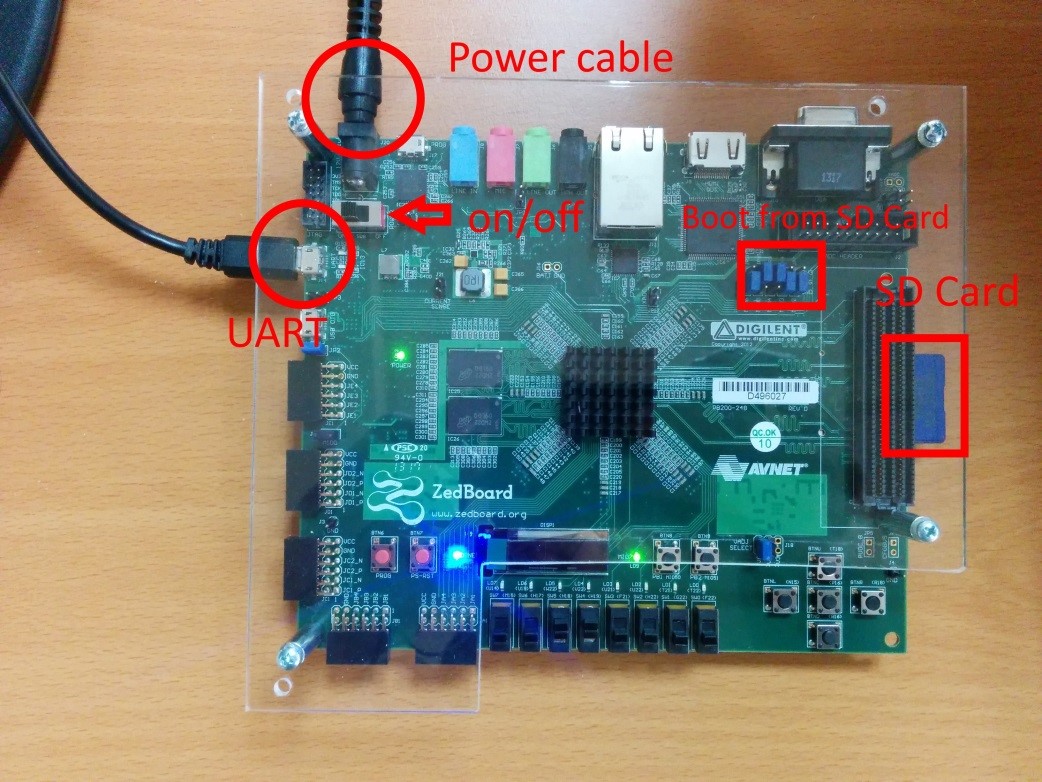
Figure 5.6 Main Zedboard components#
5.5.2.4. Set-up the terminal#
Retrieve the USB to UART COM port by opening Windows’ Device Manager:
Click Start
Click on Control Panel
In the Control Panel, click on Hardware and Sound
Under Devices and Printers, click on Device Manager
Expand Ports (COM & LPT) and locate the entry USB Serial Port (COM<X>)
Take note of the COM port as in Figure 5.7.
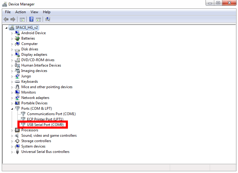
Figure 5.7 USB Serial Port#
Once the board has been powered on, PuTTY, a widely-used command-line client, must be configured as shown in Figure 5.8:
Select Serial as Connection type
Specify the COM port noted in the preceding step in the Serial line field
Speed (also called “baud rate”) should be 115200
Click Open when properly configured
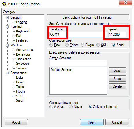
Figure 5.8 PuTTY configuration#
5.5.2.5. Launch the application#
When the terminal is successfully connected to the board, the PuTTY configuration window should dissapear. You may then turn the ZedBoard off and back on . As shown in Figure 5, PuTTY will open a command-line window where the board’s boot process will be printed. At the end of the boot process, the prompt # should be displayed. To launch the application, execute the application by typing ./zynq_apu0.core0.arm_a9.elf
When the application is started, it is waiting for user input. Simply type a valid command (i.e. 1+5) followed by a line feed (ENTER). The result of the supplied operation will be printed on the console. Refer to Figure 5.9.
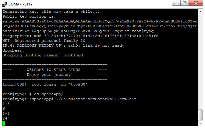
Figure 5.9 Running application#
5.5.2.6. What just happened ?#
SpaceStudio has created a Vivado project and performed all the steps needed for the bitstream generation. SpaceStudio, through Architecture Implementation technology, has generated all the required files, glue logic, firmware, Linux Drivers and has correctly configured all the cores to work together. In particular, the Architecture Implementation process has transparently implemented the adder and divider modules as hardware modules.
Communication has been refined through hardware components (such as processor_fifo_adapter & processor_fifo). These hardware components connect to the interconnect. The software modules communicate with these hardware component using optimized drivers.
Once the FPGA was programmed, a terminal was used to communicate with the application running on the FPGA.
5.6. Result files#
SpaceStudio Project