1. Architecture Exploration and Hardware/Software Partitioning

1.1. Required Files

SpaceStudio Project

1.2. Goal

The aim of this tutorial is to familiarize users with the SpaceStudio development environment to design, simulate and debug a system. You will be working with the dataflow sequence shown in Figure 1. The application is a JPEG Decoder.

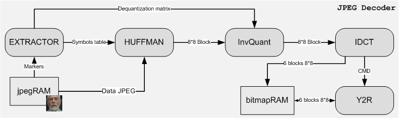
Figure 1.1 Data flow for JPEG Decoding

1.3. Target Processors

You will be working with a microblaze which is a 32-bit RISC processor that is proprietary to Xilinx. The microblaze connects to an AMBA AXI (data port) and LMB (data and instruction port) buses. The AMBA AXI serves to communicate with the peripherals and the other modules (e.g., over 2 to 3 cycles), while the LMB (Local Memory Bus) bus serves to read instructions and data directly from BRAM memory (e.g., in 1 cycle). Finally, you will see how a single task (module) runs on one or several processors, perhaps with the initial RTOS (µC/OS II) replaced by a bare-metal pseudo OS, to see how the application can be accelerated.

1.4. A few remarks before starting

This tutorial focuses on using SpaceStudio technology for architectural exploration. The hardware/software co-synthesis for implementation on FPGA (e.g., Xilinx) conducted by SpaceStudio’s Architecture Implementation feature does not play a part in this tutorial.

All of the modules for the JPEG application have been pre-characterized for timing (computation timing budget) using a high-level synthesis (HLS) tool named Vitis HLS from Xilinx. Thus, when one of these modules is mapped to hardware, SpaceStudio activates the timing models derived from that characterization. When the module is mapped to software, SpaceStudio automatically deactivates the timing annotations, since the execution time is then determined by the processor on which the module runs.

Note

In SpaceStudio, the computation timing budget is modeled by the hw_compute_latency() statement

It is possible that when you try an initial solution using multiple processors (e.g., sections 4.8), the speed-up versus a uniprocessor solution is smaller than expected. That is simply because the achievable speed-up is limited by the algorithm’s sequential fraction, and by communication and synchronization delays between processors. To achieve higher speedups, it might be necessary to make modifications to the algorithm to take further advantage of parallel computation, which this tutorial does not do.

1.5. Architecture editor

The principal view of SpaceStudio is the Architecture editor. This editor is a block design graphical interface. The Architecture editor is completely interactive: it is therefore possible to view the system, the connections and quickly configure the boxes as required. In addition, it offers more flexibility on architectural choices (i.e., connect a master interface to a free high-speed interface of the Zynq UltraScale+). This editor is familiar to system designers since it shares the same principal of downstream EDA tools (i.e., MathWorks Simulink, Xilinx Vivado, etc).

Moreover, several diagram can be open. This enables system designer to work on an architecture while another is building. The last active diagram is associated with the quick button in the toolbar.

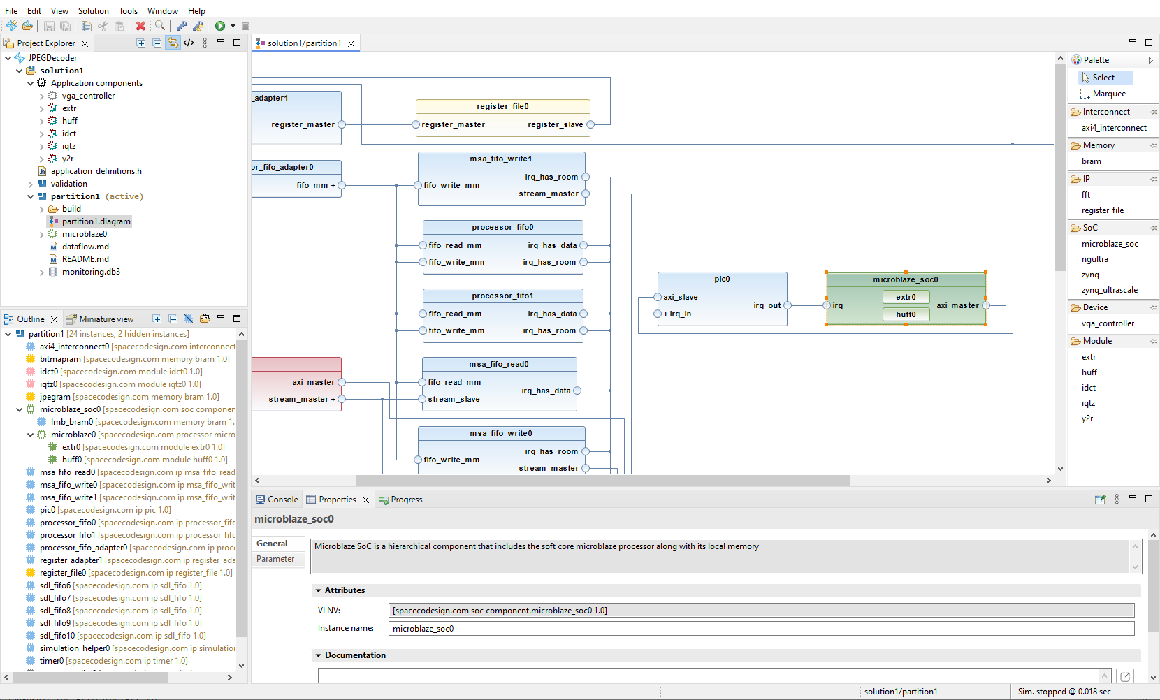
Figure 1.2 SpaceStudio

1.5.1. Color scheme

Blocks in the SpaceStudio diagram are colored according to their type, as follows:

Color	Description	Example
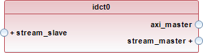
Red	Module mapped to hardware
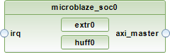
Green	Processor or module mapped to software
Gray	User-defined device
Blue	Component instance added automatically by SpaceStudio
Yellow	Component instance added manually by the user that is neither an application component or a processor

1.5.2. Action on double-click

Double-clicking on component instance will perform an action depending on the type of component instance:

• For application component instance, it will open the related .cpp file editor.

• For hierarchical component instance, it will expand/collapse the component instance

• For component instance with several ports of the same kind, it will expand/collapse all ports.

1.6. JPEG Decoder

To get started, you must first obtain a copy of the reference (initial) project. Once you have obtained the reference project, expand the zip file in a directory on a path that contains only unaccented characters without spaces. This directory will be denoted by the token %PROJECT_ROOT%.

To open the project, double-click the file JPEGDecoder.spacestudio from %PROJECT_ROOT%.

1.6.1. Functional specification

In SpaceStudio, you can create two types of design specifications: 1) functional specification (algorithm) and 2) system specification (architecture details).

The main objective of functional specification is to validate the functionality of the algorithm (does the algorithm fulfil the intended work?).

An architecture is an assembly of modules (i.e., pieces of C/C++ code) where lies an algorithm previously partitioned and library components (busses, memory, etc.) which connect these blocks together.

A functional specification is an architecture where all modules are mapped in hardware. SpaceStudio provides all the interconnects so the designers focus on the algorithm and architecture sizing.

To create an architecture:

1. Click on Solution

2. In the dropdown menu, click on New Architecture…

3. Enter validation for the name of the architecture and then click on OK

When a new architecture is created, the diagram opens. The diagram editor is the centerpiece of SpaceStudio and is used to instanciate/remove, configure instances and perform hardware/software mapping.

To configure the architecture:

1. From the newly opened diagram, uses the right pane to instanciate the following components :

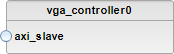
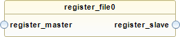
   • extr, huff, idct, iqtz, y2r and vga_controller (i.e., application)

   • register_file

2. Click on the vga_controller, go at the bottom, click on Properties tab and Parameter tab. Then, assign an addressable range of 1MB (rather than 4KB)

3. Also add 2 bram instances with the following properties (you will rename by clicking on Properties tab and on General tab, and by renaming in Instance_name):

   Instance	Memory size
   jpegram	1MB
   bitmapram	1MB

4. Preload the jpegram memory with a initial jpeg image. For the Memory initialization, click on Browse… and navigate to the folder %PROJECT_ROOT%\import and select the file jpeg_init.json. Click OK.

To execute this architecture, clicking on the run icon from the toolbar will launch the simulation.

Note

You may see an error message about a failed up-to-date check. This just means that the current output doesn’t match the latest version of the architecture. This is expected because the architecture hasn’t been built yet. To continue compiling, simply answer Yes.

To determine that the simulation is running correctly, you can check the progress messages printed in the console window, at the bottom of the GUI. The VGAController component will open a small window (128x128 pixels) that displays the decoded JPEG. This window is used to validate the decoded image. When the complete image has been displayed, it is important to close the window to finish the simulation process (right-click in the opened windows to refresh the display and show the control menu). The progress message output should appear like the following:

 -=-=-=-=-=-=-=-=-=-=-=-=-=-=-=-=-=-=-=-=-=-=-=-=-=-=-=-=-=-=-=-=
Space Codesign Systems Inc.
Copyright 2005-2024. All rights reserved
https://www.spacecodesign.com
SpaceStudio 4.4.0
-=-=-=-=-=-=-=-=-=-=-=-=-=-=-=-=-=-=-=-=-=-=-=-=-=-=-=-=-=-=-=-=
Starting simulation.
EXTR:JPEG1

Info: /OSCI/SystemC: Simulation stopped by user.

Simulation has ended @0.00073449 s
Simulation wall clock time: 0 seconds.

If you don’t see these messages, be sure to check that you had correctly followed all of the previous steps.

Note that Simulation has ended indicates the execution time for processing on image of 128 x 128 pixels, taking 0.00073449 sec. In other words, it would be possible to continuously 1361 images per second.

As for simulation wall clock time, it indicates the real-world duration of the simulation, to the second.

1.6.2. System specification (architecture details)

In this section, we will create an architecture that includes a processor. You can refine the solution for a more accurate timed design and test your application on various architectures.

1. Click on Solution

2. In the dropdown menu, click on New Architecture…

3. We will reuse the previous architecture to jumpstart the new architecture.

   1. Type partition1 as the architecture name

   2. Check the option Based on existing architecture

   3. Choose validation as the existing architecture

4. Click on OK

1.6.3. Addition of a microblaze and moving extr and huff from hardware to software

The role of extr is to read the header of the JPEG image. Since the format may evolve, extr may be updated in the future. Also, as huff is tightly connected to extr (Figure 1), we will assign extr and huff to the processor (SW partition), while the rest will stay in hardware. Therefore, using the architecture partition1, follow these instructions:

1. Open the partition1 architecture diagram

   1. From the Project Explorer, expand the partition1

   2. Double-click on the diagram named partition1.diagram to open it

2. From the diagram :

   1. From the right pane, instanciate the microblaze_soc (by dragging-and-dropping)

   2. Increase the memory size of the microblaze for the software code to 128KB by clicking on the Properties tab and Parameter tab, and by modifying the Memory_size

   3. Move the module instances huff and extr (from hardware) to the microblaze_soc (to software). This is achieved by dragging the module instance design block to the microblaze_soc design block.

To execute this architecture, clicking on the run icon from the toolbar will launch the simulation.

Note

SpaceStudio examines the application’s code to figure out how it needs to communicate. It then adjusts the platform’s hardware (adding, removing, or changing parts) to make sure the application works as intended.

It should take around 0.0186641 seconds to decode one image (Simulation has ended), or about 54 images decoded per second continuously.

Remember to close the displayed window (128x128) to end the simulation.

Warning

In Linux, clicking on the X does not work. You must exit the window by pressing the ESC key.

Repeat this section’s steps, but this time move huff to hardware and change the operating system of the microblaze from uC/OS-II to Baremetal. You should see a significant acceleration in decoding. Why?

1.6.4. Monitoring of a system architecture with 1 microblaze

1.6.4.1. Running monitoring

Next, you must execute the simulation with the monitoring feature enabled:

1. Click the arrow next to the run icon from the toolbar

2. From the dropdown, click the icon

Important

It is important to let the simulation finish on its own to ensure that it saves the data created for performance profiling. Once the simulation finishes, a monitoring.db3 node will be added to your Project Explorer.

1.6.4.2. Viewing processor load

Now that the monitoring database file is generated, manually expand monitoring.db3 > Processor load > microblaze0. Now double-click the core0 node to open the monitoring results for the Microblaze’s core 0. An example output is represented in Figure 1.3.

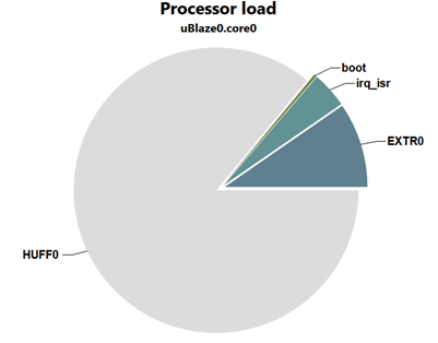
Figure 1.3 Task Profile for microblaze0

Hovering any of the pie chart’s slices will reveal a textbox displaying more precisely the proportion of execution time of that slice.

1.6.5. Hardware/Software Co-debugging

In this section, we will perform hardware/software co-debugging. During this exercise, we will examine hardware/software communications - in this case, communication between the huff and iqtz modules. For this section, we will continue working with the architecture partition1 created in the previous section. (If that architecture does not exist, you will need to create it using the previous instructions.)

Before starting, make sure the partition1 diagram is opened.

Next, you must execute the simulation with the debug feature enabled:

1. Click the arrow next to the icon

2. From the dropdown, click the icon

Once you have launched the co-simulation, a pop-up window titled Confirm Perspective Switch will appear, asking for approval to change the window layout on SpaceStudio. Select Switch to change to the debugging perspective.

Note: SpaceStudio generates an optimized version of modules which include low-level drivers for communication with the system. It is the generated files that are compiled and suitable for debugging. For instance, SpaceStudio is not debugging the iqtz.cpp file but a compiled file that will be typically named iqtz0.cpp. These generated source codes are located under the build node in the project explorer. Editing the generated files will not change the original file.

We will focus on a blocking message-passing communication between modules huff and iqtz, when the huff module writes a block of data to iqtz.

At the start, the debugger perspective only shows the hardware portion of your design architecture as shown in Figure 1.5. At this point, you can only insert breakpoint into a hardware-mapped module or user-defined device.

To insert a breakpoint into the iqtz module:

1. From the Project Explorer, navigate in partition1 -> build -> module-> iqtz0

2. Double-click the iqtz0.cpp to open it.

3. Insert a breakpoint to the ModuleRead instruction near the line 134 (as shown in Figure 1.4), with a double left mouse-click. You may need to activate line numbering in the editor window ; do a right-click on the grey space left of the editor and select Preferences, then search for Show line numbers, click the appropriate checkbox, apply and close.

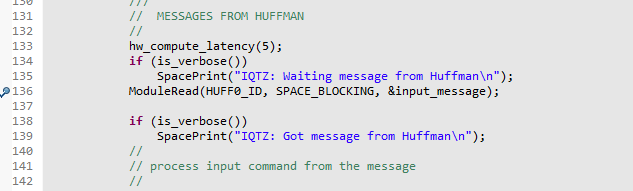
Figure 1.4 iqtz0 breakpoint

Next, start the hardware simulation by clicking on the button, i.e., Resume (F8). All the components will activate including the MicroBlaze processor model, which launches the processing of the software modules.

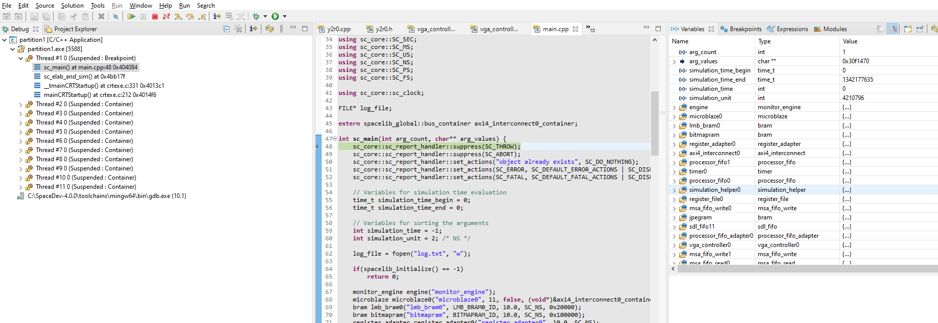
Figure 1.5 Hardware breakpoint hit

The debug console window will change, as seen in Figure 1.7, when the GDB server appears for the software execution.

At this point, you can insert breakpoint into a software-mapped module.

To insert a breakpoint into the huff module: 1. From the Project Explorer, navigate in partition1 -> microblaze0 -> build -> module -> huff0 1. Double-click the huff0.cpp to open it. 1. Insert a breakpoint to the ModuleWrite instruction near the line 134 (as shown in Figure 1.4), with a double left mouse-click. You may need to activate line numbering in the editor window ; do a right-click on the grey space left of the editor and select Preferences, then search for Show line numbers, click the appropriate checkbox, apply and close.

Select the tab for the file huff0.cpp and then insert a breakpoint near line 352 with a double left mouse-click, at the ModuleWrite line (as shown in Figure 1.6). This breakpoint will be activated when the software execution reaches that instruction.

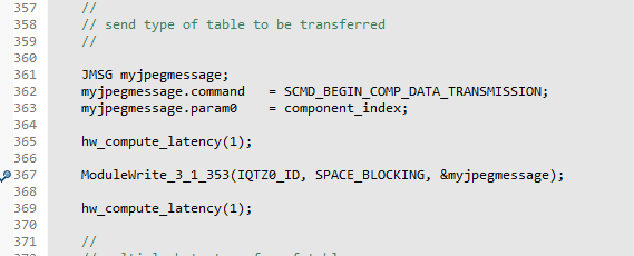
Figure 1.6 huff0 breakpoint

Right now, there are 1 hardware breakpoint and 1 software breakpoint for the matching blocking communication. We thus should expect a kind of “ping pong” mechanism when stepping through the debugging session.

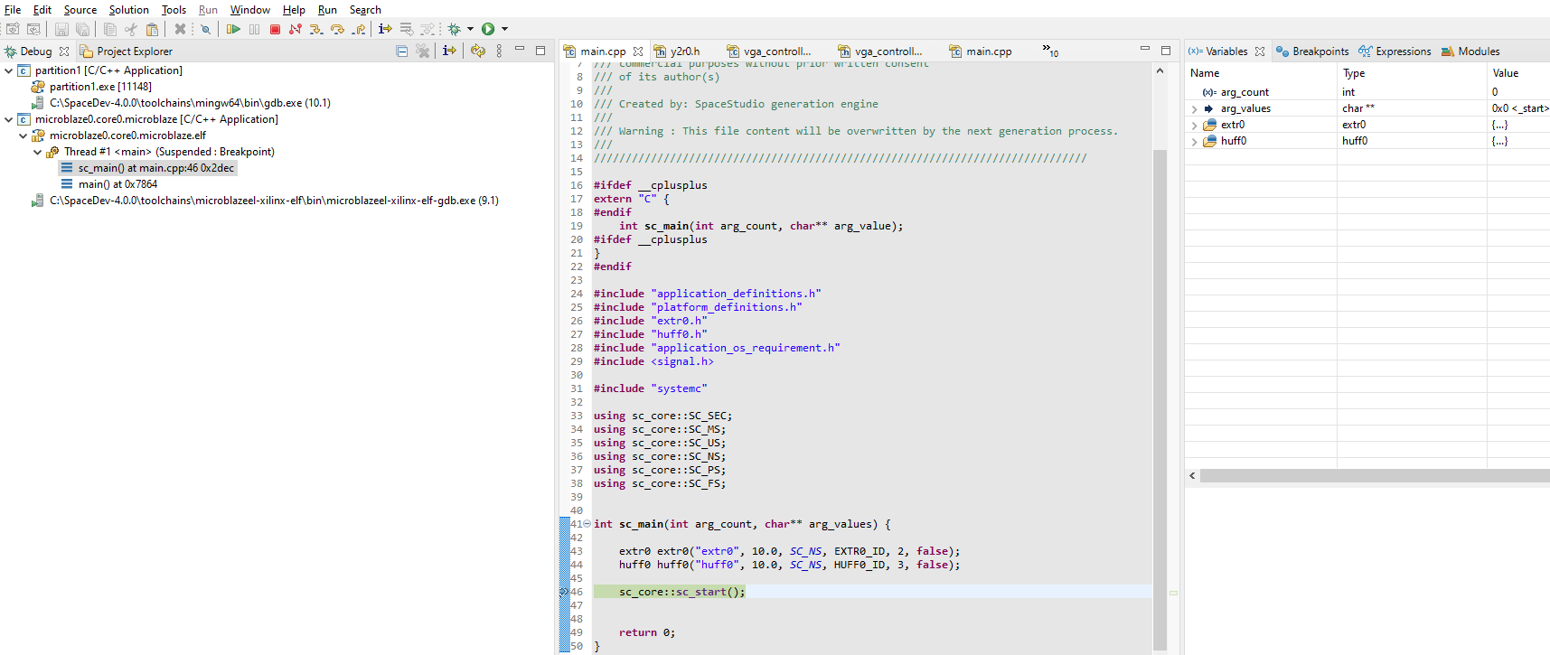
Figure 1.7 Software breakpoint hit

At this point, the hardware debugger is running while the software debugger is suspended. To resume the software debugger, click on the button to resume the whole simulation. The control of the simulation should then pass to the hardware debug window.

It is very important to understand that one window is active at a time (software or hardware). You can thus advance in the simulation (e.g., step, continue or next) one window at a time (e.g., hardware) while the other is blocked (e.g., software). Whenever you arrive at a communication by ModuleRead (or ModuleWrite), the simulation may change windows. For example, if iqtz performs a blocking ModuleRead for data not yet received from huff, it will wait until a matching ModuleWrite by huff is completed before continuing. As a result, if iqtz is executing in hardware and it becomes blocked by a blocking ModuleRead, the hardware window becomes blocked as the software window takes over to carry out the communication (i.e., the transfer of data).

At this moment, your simulation should be at iqtz breakpoint (hardware window). Click on the button and you should see control pass to _huff_ (software window). Do it again , and you should arrive at huff breakpoint. Then click again on and you will return to iqtz breakpoint (hardware window). And so on.

To summarize, each time that the thread huff executes (as a task on µC/OS II) the software module sets itself up to send data to the hardware module. By clicking on the button, that has the effect of unblocking the hardware module once it receives its data. You can then observe that the communication is blocking and that the execution of ModuleWrite has the effect of unblocking the module that carries out reading the data using ModuleRead.

This example illustrates how hardware/software co-debugging can be used to investigate the interactions between hardware and software modules. In the embedded systems industry, this approach is often called hardware/software co-simulation. To exit the simulation, you can remove all breakpoints and resume the simulation, or you can simply stop the debugging session by clicking on .

1.6.6. Creating a system architecture with 2 microblazes

We will move away from partition1 which used one microblaze and create partition2 which contains two microblazes:

1. Click on Solution

2. In the dropdown menu, click on New Architecture…

3. We will reuse the previous architecture to jumpstart the new architecture.

   1. Type partition2 as the architecture name

   2. Check the option Based on existing architecture

   3. Choose partition1 for as the existing architecture

4. Click on OK

To configure the architecture:

1. From the newly opened diagram, uses the right pane to instanciate a microblaze_soc

2. Move the iqtz0 module instance on the newly create microblaze_soc

Next, you must execute the simulation with the monitoring feature enabled:

1. Click the arrow next to icon

2. From the dropdown, click icon

Once the simulation finishes, a monitoring.db3 node will be added to your Project Explorer. Expand monitoring.db3 > Processor load > microblaze0 and monitoring.db3 > Processor load > microblaze1. Now double-click the core0 node under microblaze0 and core0 under microblaze1 to open the monitoring results for both Microblazes’ core 0.

You will see that only one task runs on microblaze1. You can thus experiment with using the bare-metal OS. Perform a new generation, compilation, execute the simulation and indicate the difference compared to a solution using uC/OS-II.

Finally, compare your simulation time (Simulation has ended) with that from the partition1 architecture from earlier. Note that you now have 50% of the application in software. Also examine the load on the processors, where there is a chance for future updates…

1.7. Result files

SpaceStudio Project